Visualization
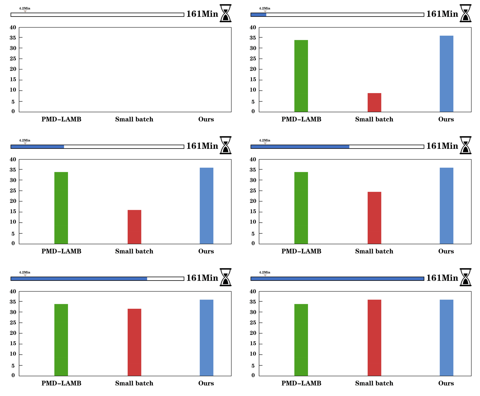
We visualize the training process of Faster R-CNN (left) and UniNet-G (right). We evaluate the detectors on COCO validation set and report the training time of 12 epochs on Faster R-CNN. AGVM can achieve 36.6 mAP with batch size 1536 within 12 epochs while PMD-LAMB only achieves 33.5 mAP on Faster R-CNN.
Highlights
We also try to push the frontier of large batch size in dense visual prediction tasks. Without bells and whistles, the batch size on RetinaNet (left) is successfully scaled to 10k with reasonable performance by AGVM, while PMD-LAMB fails (“NaN”).
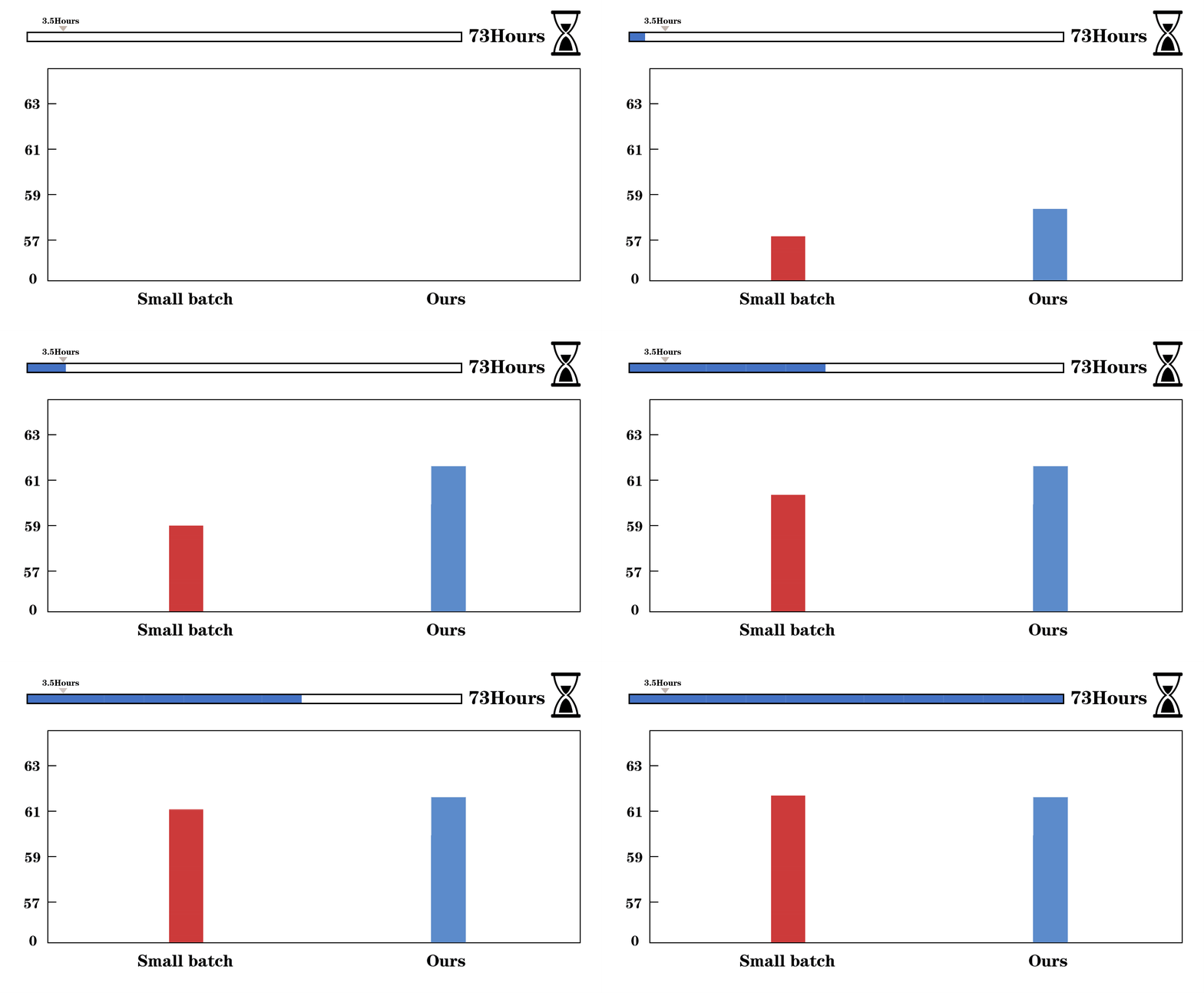
Furthermore, we evaluate AGVM on an extremely-large detector with one-billion parameters using the UniNet (right). AGVM still stabilizes and accelerates the training process in such a large model regime. But both AdamW and PMD-LAMB diverge in the early training stage.


Motivation
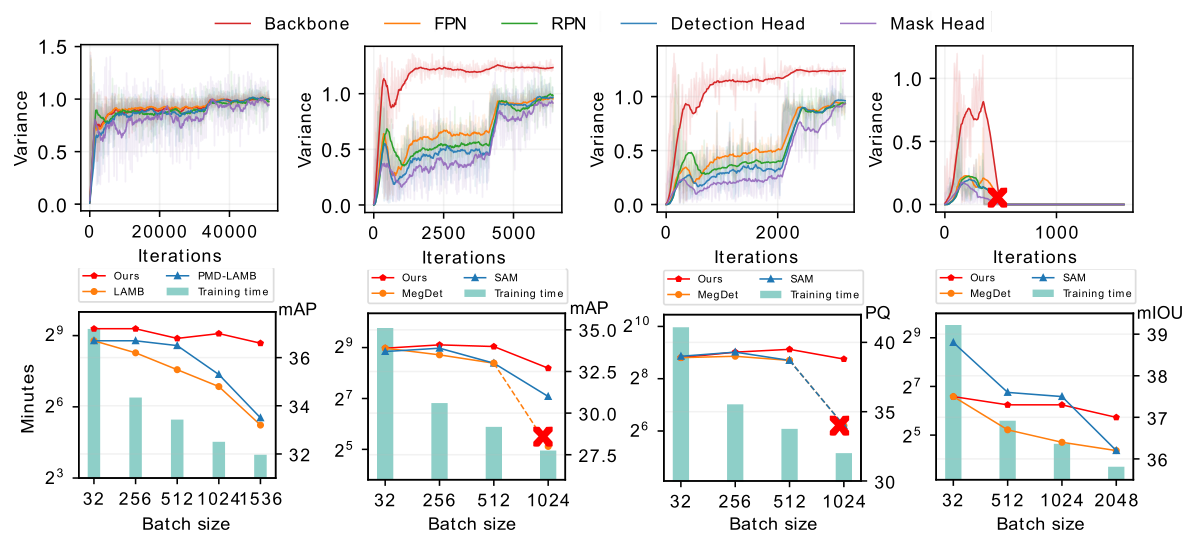
First, we give the comparisons of the gradient variances of different network modules in Mask R-CNN, including backbone, FPN, RPN, and heads. From the left to right, the models are trained using SGD optimizer with a batch size of 32, 256, 512, and 1024. When batch size increases from 256 to 1024 (2nd~4th figures in the first row), the gradient variances suffer heavy misalignment between different network modules. In the second row, we show our method outperforms the recent approaches in all tasks, significantly reducing training time.
Comparisons of Variances in Different Pipelines
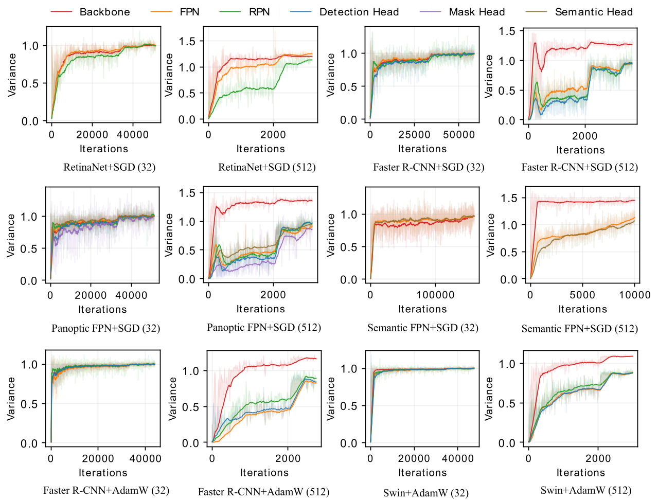
In the following, we give an overview of variances of different pipelines (i.e., RetinaNet, Faster R-CNN, Panoptic FPN, and Semantic FPN) and different optimizers (i.e., SGD and AdamW). The number in the bracket represents batch size. All pipelines use ResNet50 as the backbone network other than the last two figures, where we adopt Faster R-CNN+Swin-Tiny to visualize the variances.
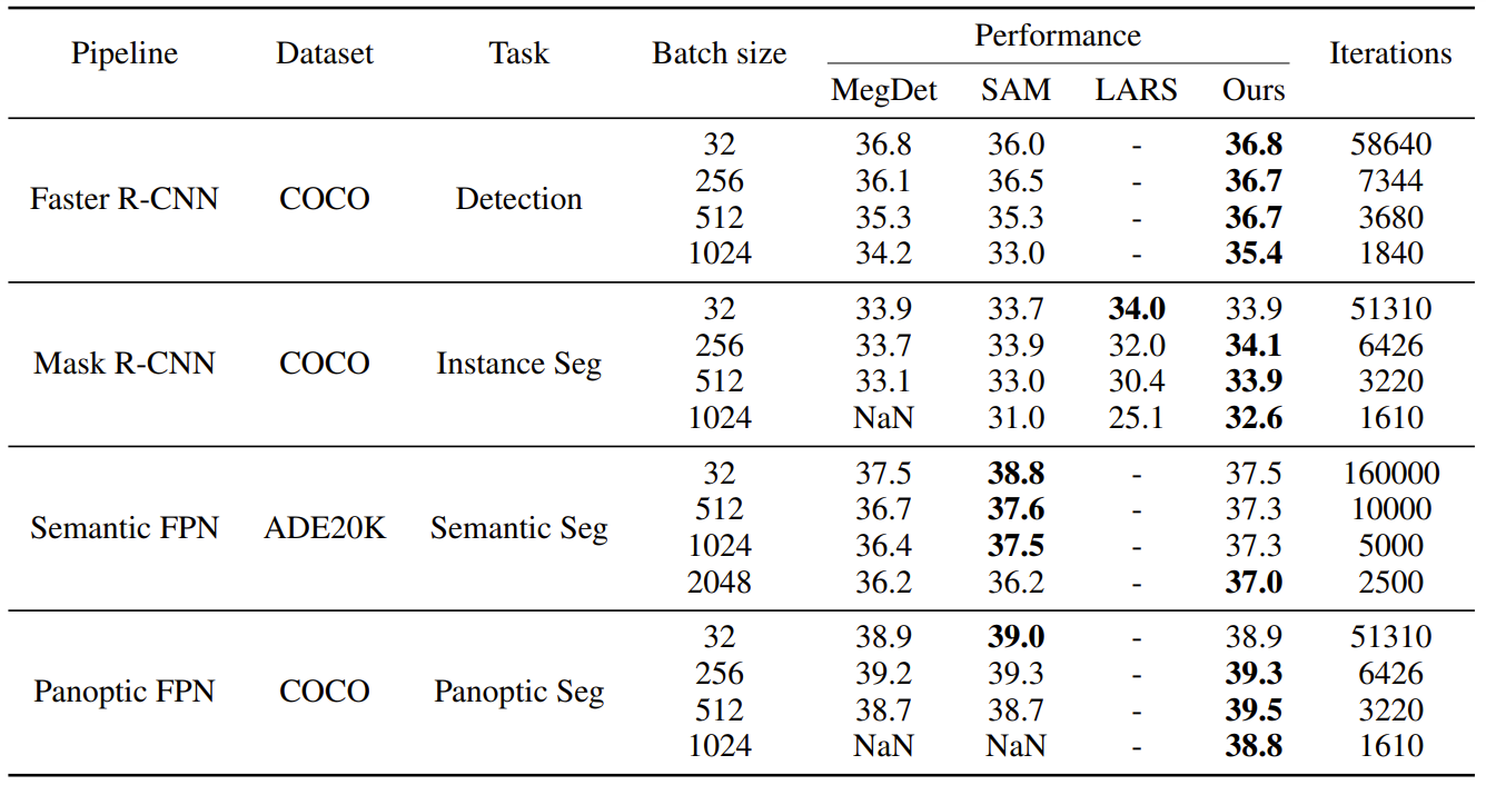
Performances on Various Tasks
We give the comparisons of performances in different tasks (i.e., object detection, instance segmentation, semantic segmentation, and panoptic segmentation). All visual predictors are evaluated on the validation set. We use SGD as the optimizer and see that previous methods’ performances drop a lot when scaling the batch size and even result in training failure when the batch size is 1024 (“NaN”). The best-performing models are shown in bold.
Codes and Models
Coming soon!